How to use lookup in Excel (and Jotform Tables)

Working with a spreadsheet can feel like combing through the ultimate haystack, with so many needles to find. Sometimes, locating a particular piece of data is critical, but trying to extract it from the mass of rows and columns is just too big an ask.

That is, until you discover the lookup feature.

Lookup is a formula that works in Excel and other spreadsheet programs, helping locate a particular piece of unknown data that relates to a piece of known data. For example, say you know the name of a product, but you don’t know the corresponding SKU. Or perhaps you want to find out which salesperson was responsible for taking a particular order.

We’ll use the latter example to explore how to use lookup in Excel. Here’s how to get started.

1. Identify the data you want to look up

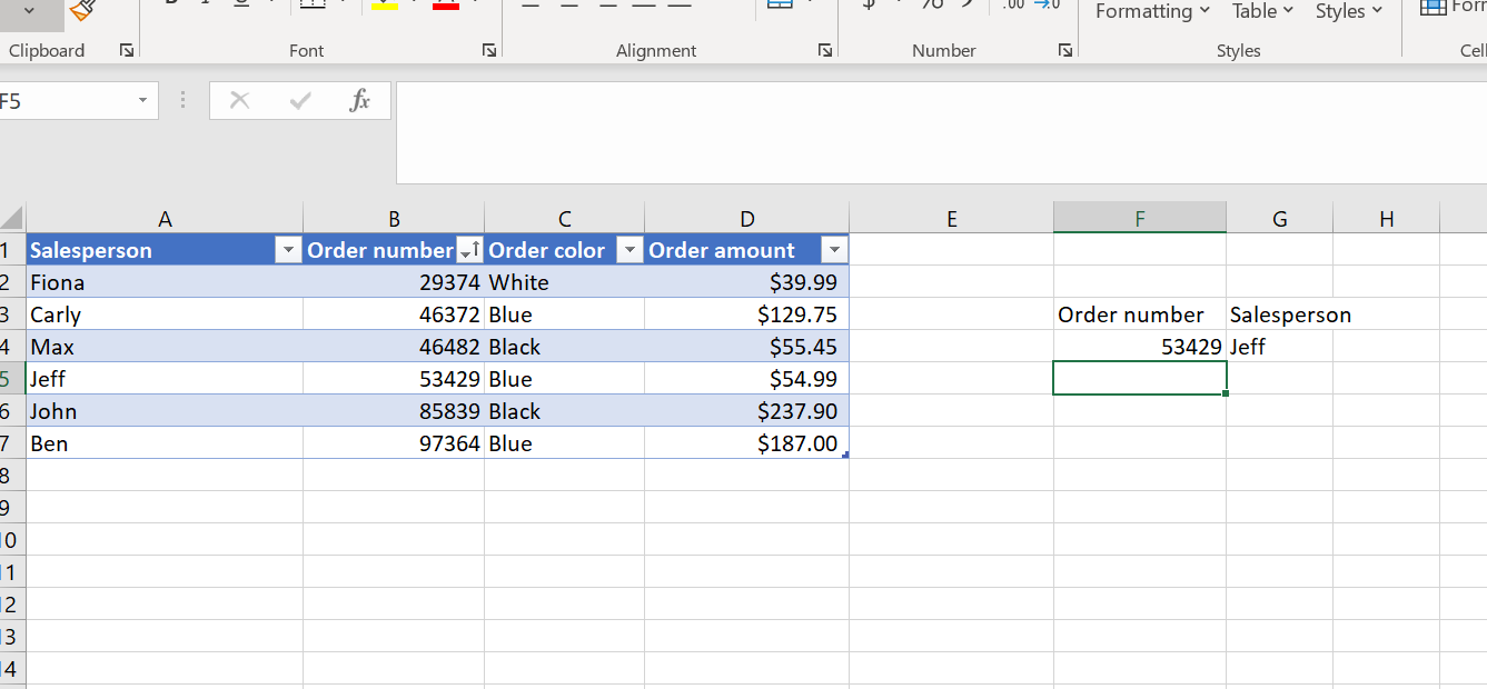
First, decide what data you’re looking for. In the example spreadsheet below, we want to find out which salesperson is responsible for a particular order, based on the order number.

Pick a couple of cells outside of the table, and name them according to the value you want to look up (order number) and the value you want the lookup to provide (salesperson).

2. Enter the data value for the lookup

In the order number lookup cell, enter the value you want to search for. In this instance, we want to find out which salesperson took order number 46482.

3. Create the lookup formula

Place the cursor in the cell where you want the lookup result to appear — in this case, the salesperson field. Now we’ll enter the following formula:

=LOOKUP(lookup_value, lookup_vector, [result_vector])

Here’s the formula explained:

• Lookup value: This is the data you’re basing the lookup on — in this case, order number 46482.
• Lookup vector: This is the data column where the lookup value should be searched for — in this case, column B (order number).
• Result vector: This is the data column where we want the result to be found — in this case, the salesperson list, which is column A.

To create the lookup formula, click on the cell where the result (salesperson name) will appear.

Excel formulas begin with an equal (=) symbol, followed by the formula name, a parenthesis, the formula data separated by commas, and a closing parenthesis.

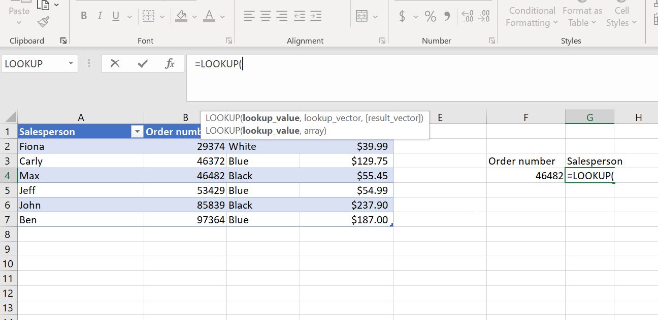
To use lookup, begin typing the formula like this:

=LOOKUP(

Now we can enter the values in the formula.

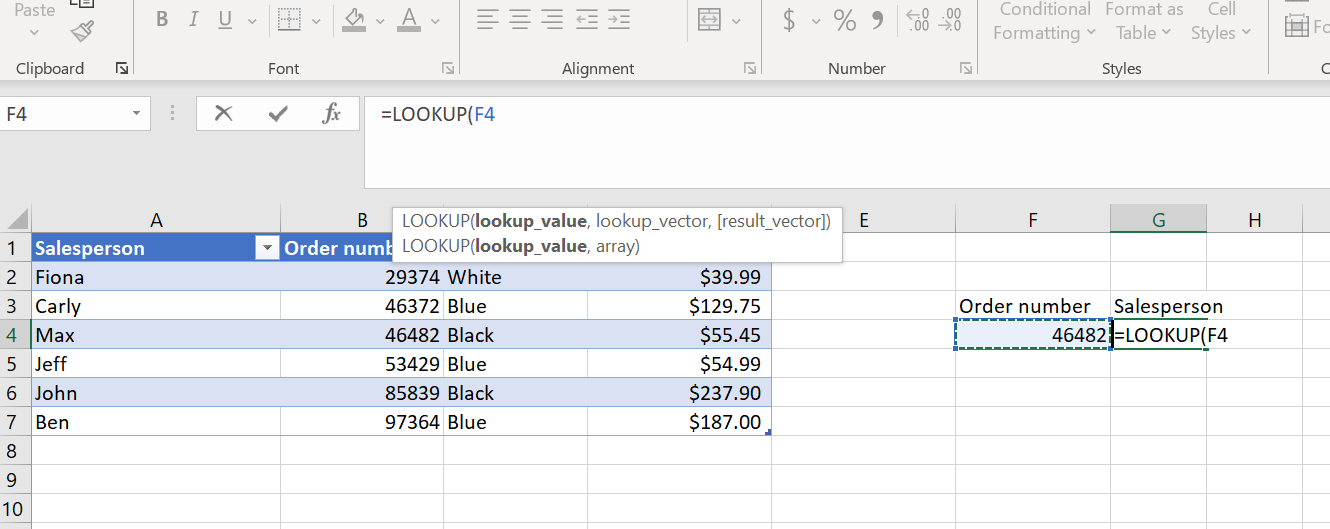
You entered the lookup value (order number) in cell F4. Click on that cell, and it will automatically insert the cell name into the formula.

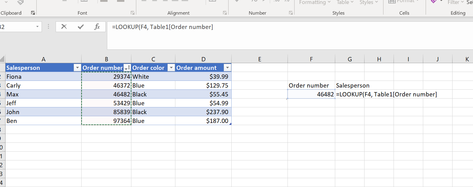
Next, add the lookup vector, or the data column where the lookup value is located — in this case, the order number column. Add a comma, then select the order number column. The cell range of the order number column is automatically inserted in the formula.

Add a comma, and insert the result vector, the data column from which the result will be sourced, in this case, the salesperson column.

End the formula with a parenthesis, and press enter.

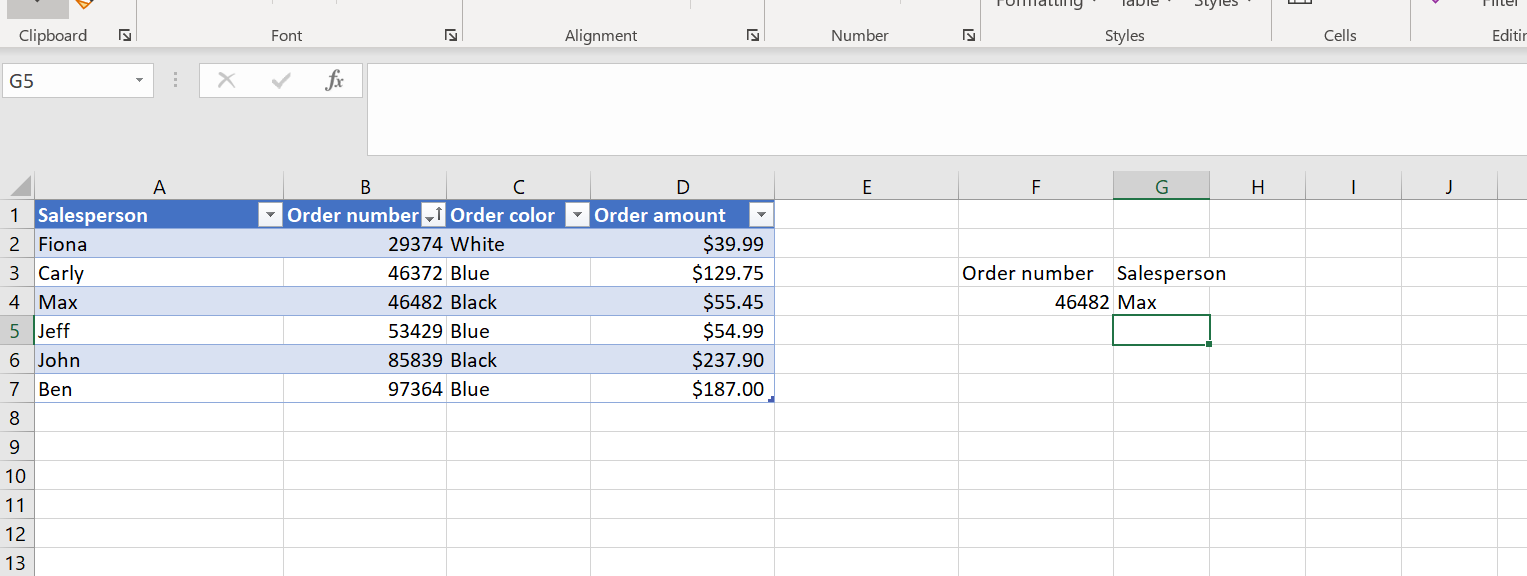
As you can see, the lookup formula has successfully identified the salesperson corresponding to order number 46482: Max.

4. Use the formula for more lookups

To look up any other order number, type it into the lookup value cell and click enter. The salesperson listed in the table for the order number will automatically appear.

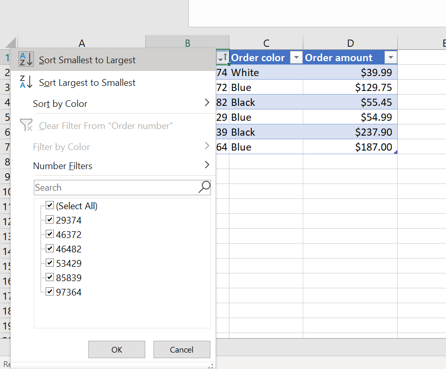
The data in the lookup vector column must be sorted from the lowest to the highest value for the formula to work. In this example, the lookup vector column is the order number column.

To sort the column, click on the dropdown arrow on the right corner of the column header cell, select sort smallest to largest, and click OK.

Creating a lookup formula in Jotform Tables

The lookup formula feature in Jotform Tables is conveniently available from the column creation function.

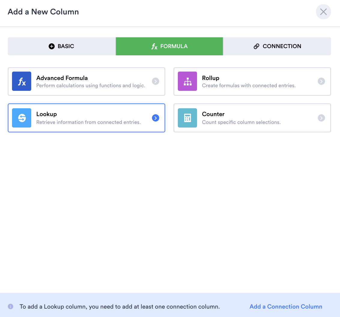
To add a lookup column, click +Add in your table. Click the Formula tab in the Add a New Column dialog box, and select Lookup.

Next, add a connection column from which lookup data can be retrieved. Follow the prompts in the Jotform Tables wizard to connect the column via a form or a table. Enter the name for your lookup column, then choose the form or table and the specific reference column for the lookup data.

At this stage, you can decide whether to allow multiple options to be selected for each row and whether you want to set an automatic default value for the cells. Click OK, and your lookup column is ready to go!

Your spreadsheets are looking up

Lookup is an easy and useful tool to mine your data for corresponding entries. There’s no need for time-consuming manual scanning. Using lookup in Excel and Jotform Tables, you can extract much more from your spreadsheets — and get data that will keep your business operations on the up and up.